Decision Tree
Decision Tree is a supervised machine learning model, that can handle both regression and classification problems. It is a non-parametric method which makes it very versatile. The tree makes decisions which mirror human decision thought process so can be easily interpreted.
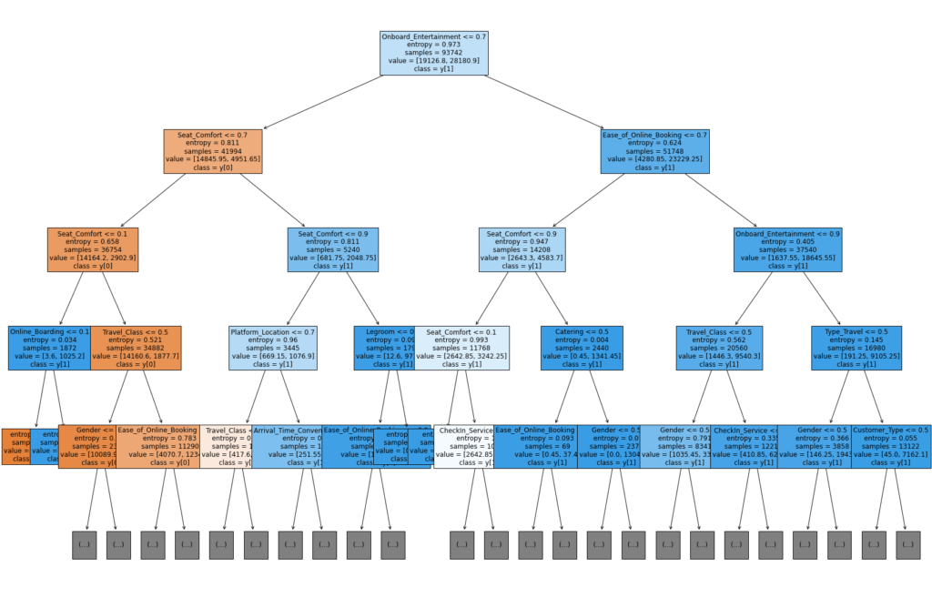
A tree is comprised of nodes, branches, and leaves. Except for the leaves, every node in a tree is a decision node that splits data into further sub-nodes. Each leaf represents a class label. The length of the longest path from root note to leaf is the depth of the tree. The below tree has a depth equal to 4.
A decision tree finds the optimal split of features based on gini impurity or entropy, they are functions to measure the quality of a split.
Gini Impurity
Mathematically expressed as:
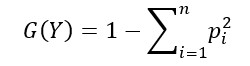
where Y is the target variable and pi is the probability of ith class in the data
The value of gini impurity ranges from 0 to 0.5. The minimum value of 0 happens when the node is pure and all data in the node belongs to the same class. The maximum value happens when the probability of the classes is equal.
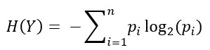
Entropy
I first learned about entropy back to the time in university when I studied thermodynamics. Unlike the second law of thermodynamics states that the entropy of an isolated system can only increase, it can decrease in the field of information theory. Entropy is a measure of randomness or impurity contained in data. Mathematically, it is written as:
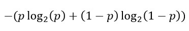
Let’s consider a binary event such as coin tossing or whether the sun will rise tomorrow. The probability of one outcome is p and the probability of another is 1-p. The entropy of this event is expressed as:
We can visualize this by plotting the gini impurity/entropy against the probability of event:
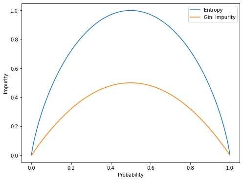
As we see from the graph, the gini impurity and entropy will be minimum when we can only get one outcome (with a probability of 0 or 1). It is said that the gini impurity/entropy will be minimum when the outcome is homogeneous. And will be maximum when the outcomes are equally likely to happen (with a probability of 0.5).
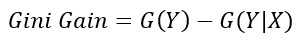
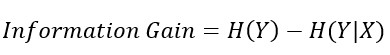
After having an idea of what gini impurity and entropy are, we can know how a node splits data. The node splits the data in a way that results in the highest purity. To know the purity, we simply subtract the gini impurity/entropy after the split from that before the split. And this gives us the Gini Gain or Information Gain.
Gini Gain = (gini before the split) – (weighted gini after the split)
Information Gain = (entropy before the split) – (weighted entropy after the split)
Notice that the gini impurity/entropy of a split will always be less than or equal to the gini impurity/entropy of the target variable, the minimum gini gain or information gain of a split is zero. This implies that the selected feature we split on did not have predictive power on the target variable.
The decision tree will run through all the input features and split on the feature that results in the highest gain, and this will be the first decision node. This is because the less impurity in a node will give the model more predictiveness. After the first split, the following decision nodes will be the feature left out that gives the highest gain subsequently. All the decision nodes follow this recursive process to split data. Without defining a maximum depth, the splitting will stop when the leaf nodes become homogeneous. Which means all the data in the leaf belongs to the same class. The decision tree locates the global optimum by finding the local optimum at each step. Therefore, decision tree is a greedy algorithm in nature.
To implement the decision tree model, we import DecisionTreeClassifier (or DecisionTreeRegressor) from sklearn.tree.
As decision trees make decisions after computing all attributes, therefore, it is sensitive to small changes in data. Usually, a fully grown decision tree is too complex and prone to overfitting.
Pruning
Pruning is a method to avoid overfitting. We can do this by tuning the hyperparameters prior to training the tree, and this is called pre-pruning. In the above tree example, we use entropy as criterion and set the maximum depth of the tree to equate to 4. There are other parameters such as “min_samples_split”, “min_samples_leaf”, “max_leaf_nodes”, “min_impurity_decrease”, etc. By specifying these parameters, our tree will stop growing before it is fully grown.
We can determine the optimal parameters using GridSearchCV to search over a range of possible values for the hyperparameters and choose the values that result in the best cross validation score.
As opposed to pre-pruning, another technique is post-pruning. We start by allowing a decision tree to be fully grown (maximum depth) and then remove some non-significant subtrees to reduce model complexity. We start at the homogeneous leaf node and work backwards by calculating the performance scores at each stage. If the subtree is insignificant, it can be replaced by a leaf and assigned to the most common class at that node.
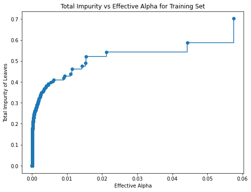
To implement post-pruning, we use a cost complexity parameter “ccp_alpha” in scikit-learn. A greater value of ccp_alpha increases the number of nodes pruned. To pick a suitable ccp_alpha value, we use cost_complexity_pruning_path( ) method of a tree object to compute the effective alphas and the corresponding total leaf impurities at each step of the pruning.
We can visualize the total impurity versus different effective alphas using matplotlib:
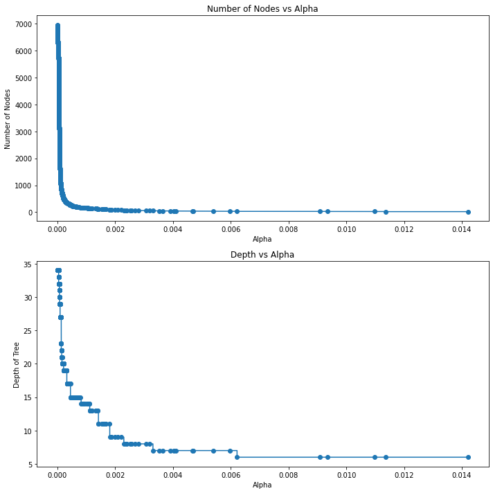
Then, we train our decision tree with the effective alphas. We can visualize the relationship between different alphas and the number of nodes and depth of the tree.
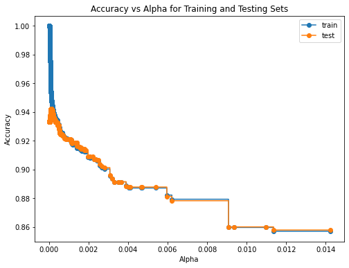
To know how our tree performs regards different values of alpha, we plot the train and test accuracy for each value of ccp_alphas.
The drawbacks of pruning are that we lost some information in the process as we removed subtrees, and the method is computationally expensive.
Ensemble Learning
The idea of ensemble learning is to combine predictions from multiple base models. Some examples of ensemble learning are bagging and random forest. Despite each of these independent models will make a certain error, the probability of the majority making a significant error is lower compared to the probability of a model making one.
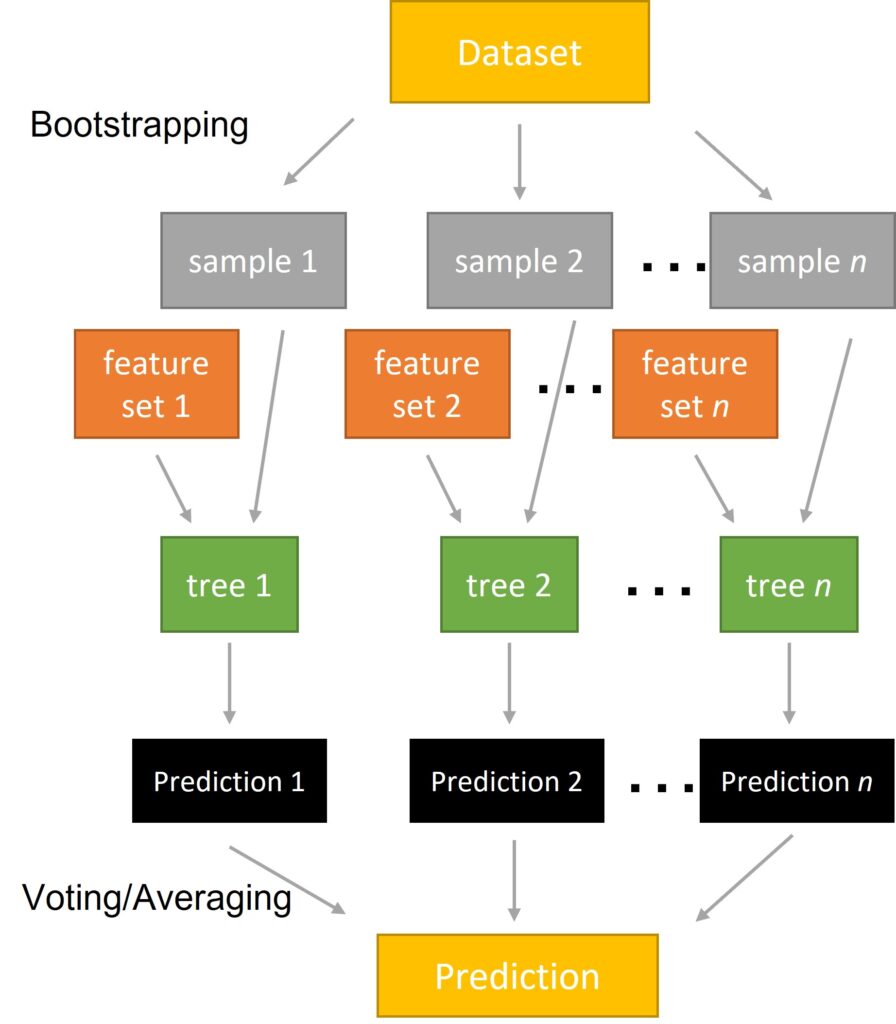
Random Forest
Random Forest is an application of ensemble learning in decision trees. It takes the average of predictions from many decision trees, and each individual tree is a weaker predictor of the full-grown decision tree. Instead of using all the features at each node, these trees are individually trained on a random subset of the original dataset with a random subset of features. By combining the trees, we can get a better performance and more stable result.
To implement random forest with scikit-learn, we instantiate a RandomForestClassifier/RandomForestRegressor object from sklearn.ensemble.
Gradient Boosting
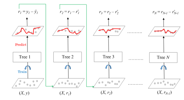
Gradient boosting uses “weak learners” (in this sense, the decision trees) combined to make a single strong learner in an iterative fashion. Each decision tree is even weaker compared to those used in random forest. The uniqueness of gradient boosting algorithm is that it adds trees sequentially and the subsequent trees built try to reduce the errors of the previous trees. This is done by updating the weights to the predicted outcomes in the previous model with their gradient of the loss function. This method is called gradient descent (we will talk about this in a separate discussion). Therefore, the model generally has a lower bias and higher accuracy compared to random forest. We can implement gradient boosting with GradientBoostingClassifier/GradientBoostingRegressor from sklearn.ensemble.
Another very powerful library for gradient boosting is XGBoost (stands for eXtreme Gradient Boosting), which is more memory-efficient and better performing compared to scikit-learn’s one.