What is logistic regression?
When we are dealing with problems that require prediction of outcomes in binary classes, simple linear regression does not suffice. Imagining that it will be hard to fit a straight line to two distinctly separate data groups. The output of linear regression is continuous and can go to infinity. Here shed light on the logistic regression.
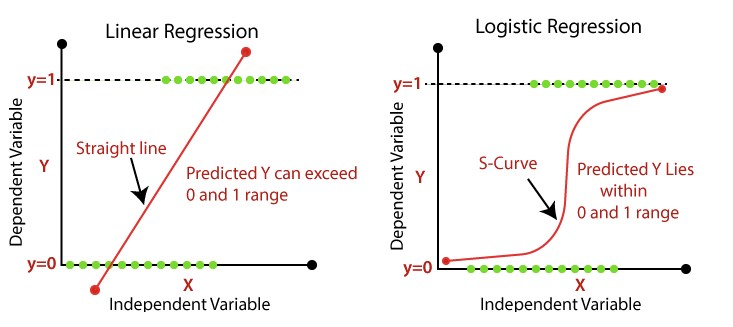
Logistic regression is a statistical method used to analyze and model the relationship between a binary response variable (a variable with only two possible outcomes) and one or more independent variables. It estimates the probability of an event occurring, as the output is a probability, the response is bounded between 0 and 1. Instead of fitting a best-fit straight line like linear regression, logistic regression fits a sigmoid function (“S-curve”) to the data. This model is widely used in various fields, such as finance, healthcare, and marketing to deal with classification problems.
Assumptions and Modelling
Before going into detail, let’s talk about some of the underlying assumptions of this model. Unlike linear regression, logistic regression requires little assumptions to begin with. First, it assumes the observations to be independent of each other. Second, it assumes there is no or little multicollinearity among independent variables (the independent variables should not be highly correlated). Third, it assumes a linearity of the independent variables and the log odds (response in the transformed linear model).
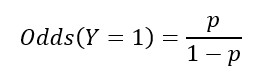
Odds are the probability of an event divided by the probability that the event will not occur.
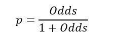
Therefore, we can work out the probability from the odds.
The logistic response function (sigmoid function) of the predictors to model probability is written as:
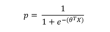
Where θ is the parameter vector and X is the predictor vector.
By combining the odds expression and the logistic response function, we can represent the log odds in a linear function of the predictors:

The logit function maps the probability P from (0, 1) to (-∞, +∞) range. And the predicted value from logistic regression is in terms of the log odds. To obtain the predicted probability of the event, we need to map the log odds back by the logistic response function.
Model Fitting – Maximum Likelihood Estimation
To find the best-fit curve, we must use the maximum likelihood estimation (unlike linear regression using the least squares). Understanding that in logistic regression, the predicted response is not 0 or 1 but an estimate of the log odds that the response is 1.
Considering we have a set of data (X1,X2,X3,…,Xn) and the corresponding probability model Pθ (X1,X2,X3,…,Xn) that depends on a set of parameters θ. Maximum likelihood estimation aims to find the set of parameters ![]() such that maximizes the probability of observing (X1,X2,X3,…,Xn) given the model P.
such that maximizes the probability of observing (X1,X2,X3,…,Xn) given the model P.
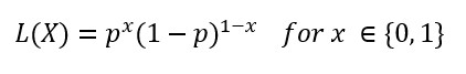
In early time, we assumed each observation of data is independent of the others. The likelihood of observing a set of data (X1,X2,X3,…,Xn) is the product of observing each independent data point in the same distribution. The likelihood for Bernoulli distribution to observe a single data X is written as:
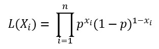
Our goal is to maximize the likelihood function that observing a set of data:
The model is evaluated using deviance:
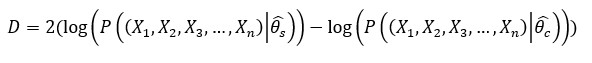
Where![]() is the fitted parameters of the saturated model and
is the fitted parameters of the saturated model and![]() is the fitted parameters in the current model. Lower the deviance means the better fit.
is the fitted parameters in the current model. Lower the deviance means the better fit.
Now we can continue the last post talking about Exploratory Data Analysis, I will demonstrate the working of the logistic regression on the Titanic dataset.
Data Preprocessing
Previously, we examined the correlation of different preditors and Survival. Here we dropped the variables that do not give us predictive power.
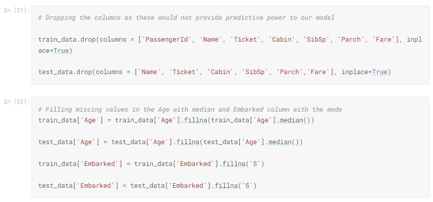

We also imputed the missing values that we found in our earlier analysis.
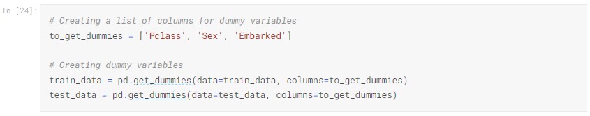
We created dummy variables for categorical variables.
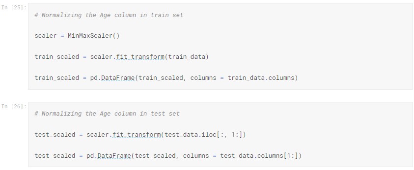
Variables usually presented in different scales. When these features have different scales, there is a chance that a higher weight will be assigned to some features that have higher magnitudes. Since these features do not guarantee significance in predicting the outcome which will bias our model. We have to normalize these features before training our model.
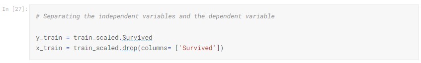
Now we split the data into dependent variable and independent variables.
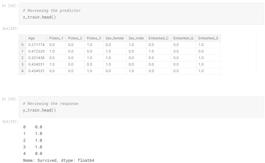
A final review on our data:
Model Building and Evaluation
We will use scikit-learn library for logistic regression. Building a logistic regression model with scikit-learn is straightforward which requires little coding. We fit our independent and dependent variables into the logistic regression object.
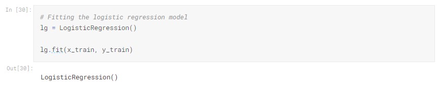
In scikit-learn, logistic regression adds L2 regularization by default.
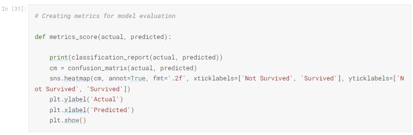
For model evaluation, here we will simply use the confusion matrix to gauge the performance of our model.
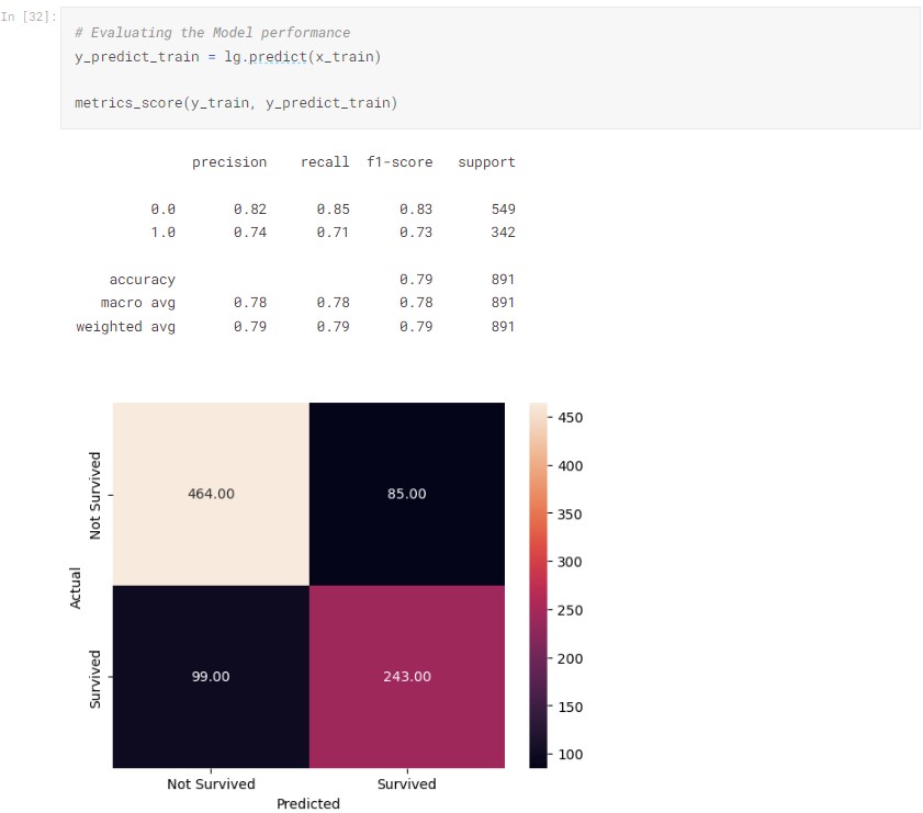
The classification report gives us different performance metrics (accuracy, precision, recall, and F1 score) derived from the confusion matrix. In this case, we are getting an in sample accuracy of 79%.
Conclusion
Logistic regression is a powerful statistical method that allows us to model the relationships between a binary response variable and one or more explanatory variables. We explored the theoretical background of logistic regression, including the concept of odds, the sigmoid function, and maximum likelihood estimation. We also demonstrated its application in Python by using it to predict the survival of passengers in the Titanic dataset.
In case you want to access the notebook and look at the code, you can click HERE.
Reference
Linear regression vs logistic regression – javatpoint. www.javatpoint.com. (n.d.). Retrieved March 27, 2023, from https://www.javatpoint.com/linear-regression-vs-logistic-regression-in-machine-learning