Exploratory Data Analysis (EDA) is an essential step in understanding the data we have in hand, so we can have a general idea of what the data is about and its characteristics (e.g., distribution, descriptive statistics, abnormalities). It’s a technique to investigate and manipulate data sets by employing visualization and summary statistics to discover hidden data patterns. Based on the known findings we can better formulate the machine learning problem and feature engineering our model. The idea of EDA was originated by John Tukey in his book “Exploratory Data Analysis” published in 1977. This technique is widely used in all data science and statistical projects.
The general process of EDA involves explaining the descriptive statistics such as mean, mode, median, variance and standard deviation. Explaining the data distribution using histograms and box plots. Finding correlation and covariance among different variables by using various plots. Identifying missing values and outliers to impute data for feature engineering and data preprocessing.
In this post, I will briefly introduce EDA by walking through one of the most overdone datasets – Titanic from Kaggle.
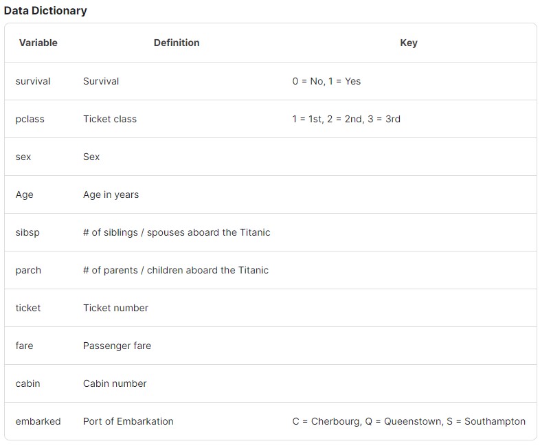
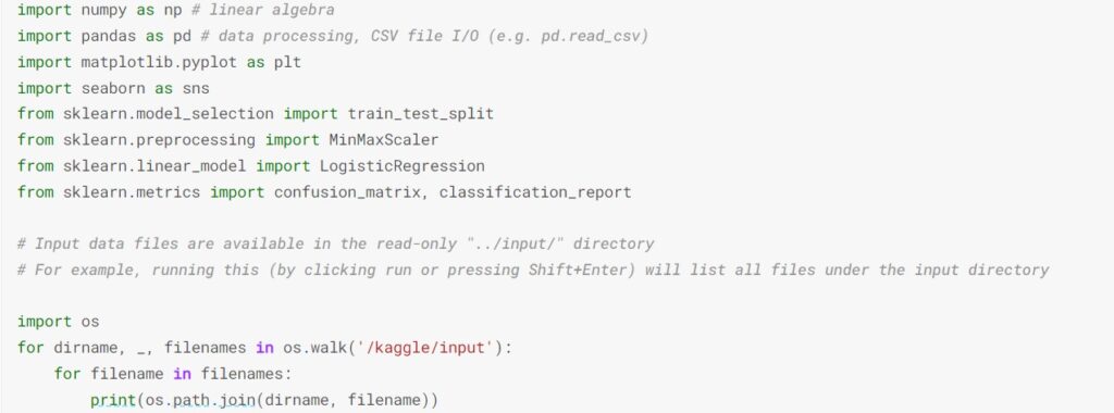
We start with importing the libraries that we will use and followed by loading the datasets into the notebook. The objective of this notebook is to explore different variables for feature selection and data preprocessing for later use. Kaggle provides two datasets – “train.csv” and “test.csv”.
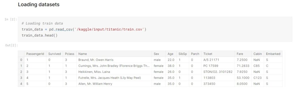
After loading the data, our first intuition is to take a glance at the first few rows of the dataset to have a rough idea of what the data is about.
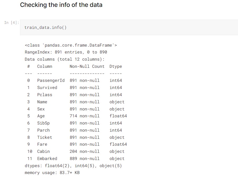
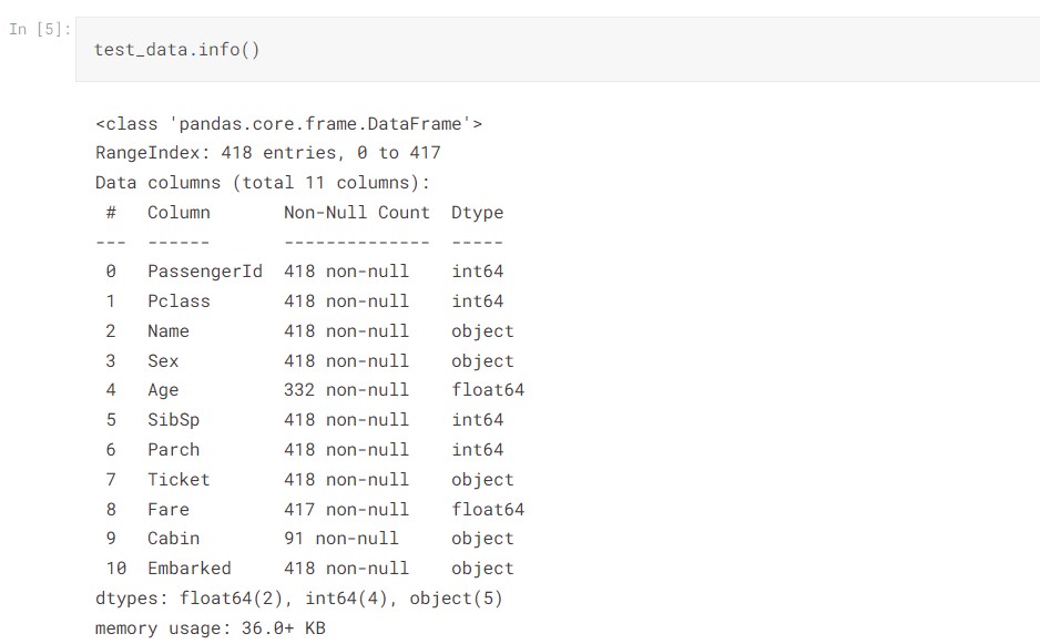
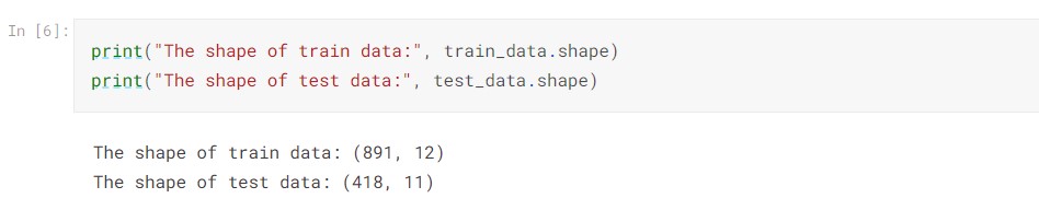
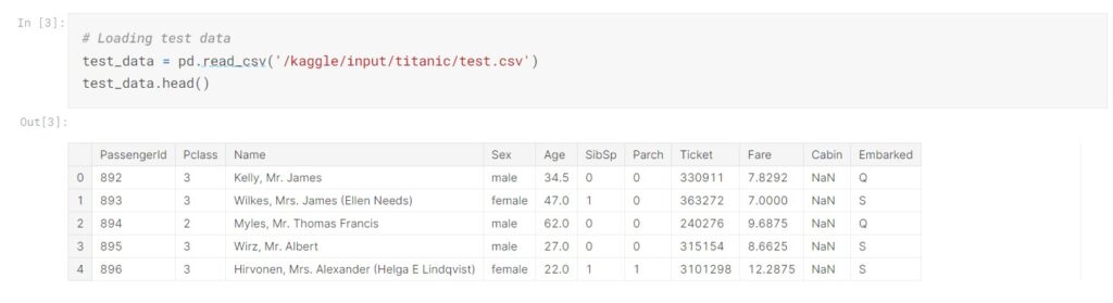
By checking the data info, we see there are 891 entries and 12 columns in the train data, 418 entries and 11 columns in the test data. The train data is the data set that we will focus on to do the EDA and further train our machine learning model. There are some missing values in the column Age, Cabin, and Embarked as their number of values are less than others.

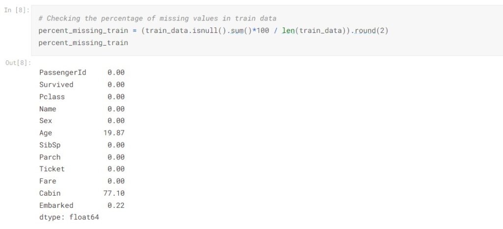
We take a closer look at the number of missing values presented in each column. In the train data, there are 19.87% of data went missing in Age and 77.10% of data went missing in Cabin. Which takes up a significant portion of the column.
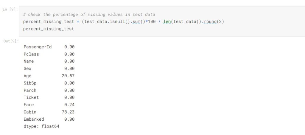
In the test data, 20.57% of the data went missing in Age and 78.23% of data went missing in Cabin, the proportion of missing values is about the same as the train data.
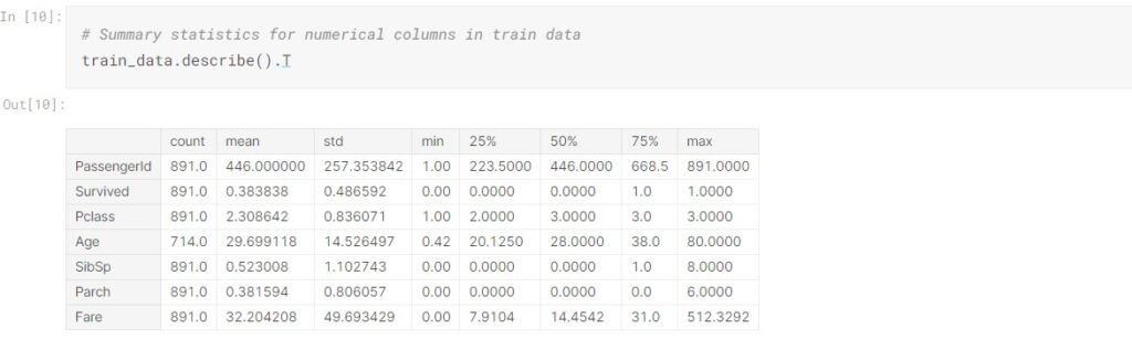
To check the summary statistics for numerical columns:
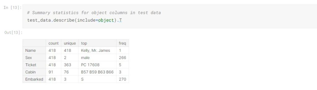
To check the summary statistics for categorical columns:
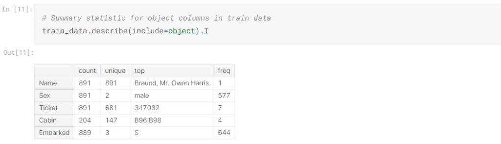
PassengerId is the primary key, and there is no duplicated entry in the dataset. Pclass is the class ticket that passengers held, it should be categorical but has been classified as numerical by default. From the summary statistics, we observed that more than 50% of the ticket class is 3rd class; the average and median age of passengers are 30 and 28 respectively. The Age, SibSp, Parch, and Fare appear to be right skewed. 577 passengers are male accounting for 64.76% and 644 passengers embarked from Southampton which accounts for 72.44%.
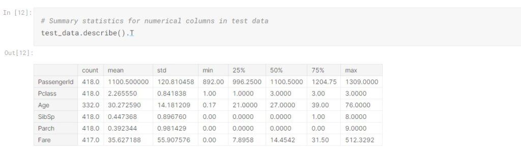
Let’s look at the test data as well:
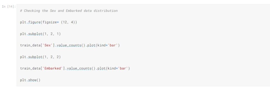
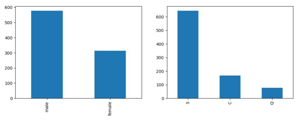
Now we examine different variables by univariate analysis. Checking the data distribution of Sex and Embarked columns by bar plot.
Now we create histograms and bar plots to explore each feature.
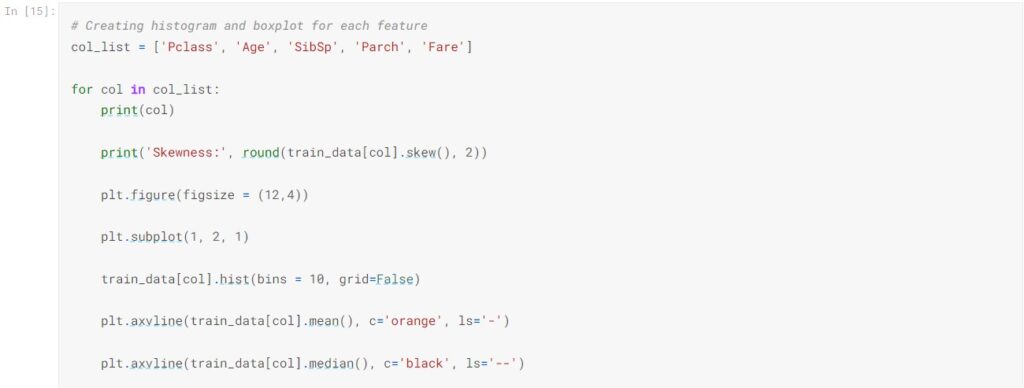
The orange line represents data mean while the dotted line represents the median.
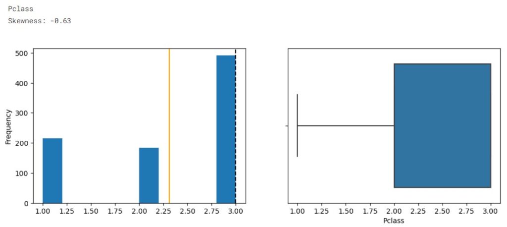
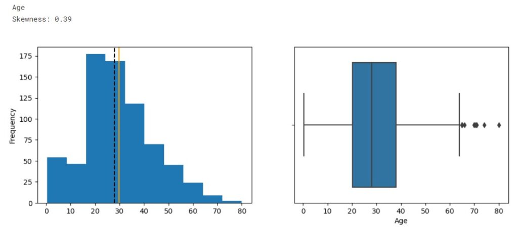
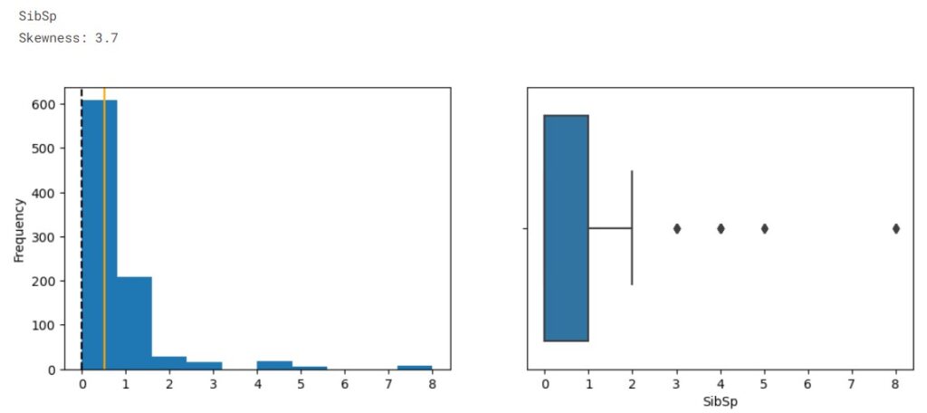

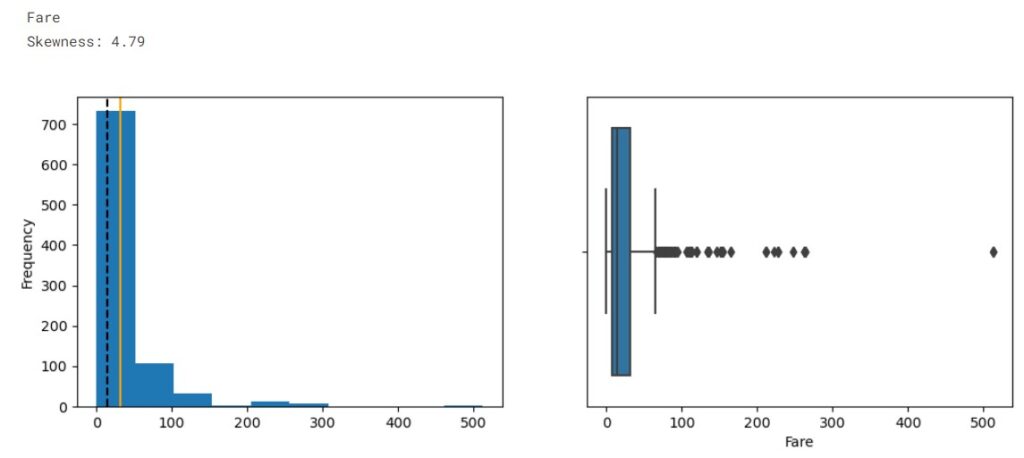
From the distribution, we observe the data is imbalanced. The plots show that SibSp, Parch, and Fare are highly right-skewed, while the Age is approximately normally distributed. From the boxplot we see outliers presented in Age, SibSp, Parch, and Fare.
Now we do multivariate analysis to explore the relationship between features.
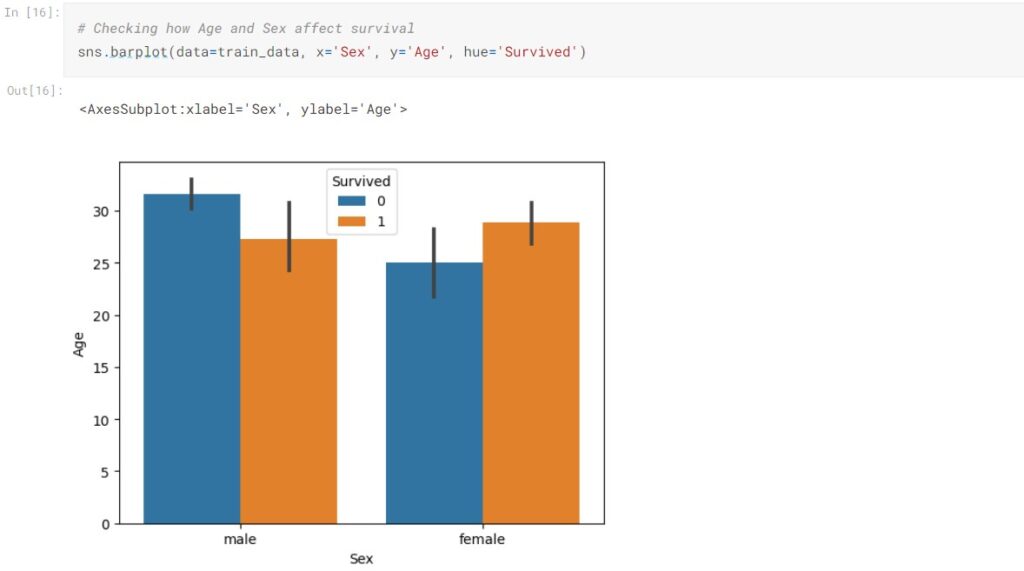
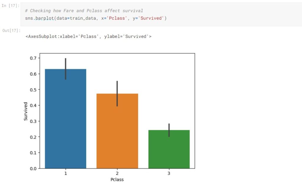
The female passengers seemingly have a higher survival rate than males. We also observed that class 1 passengers have a higher survival rate than class 2 passengers and class 2 passengers have a higher survival rate than class 3.
Let’s calculate the exact survival rates for male and female passengers to confirm our graphical observation.
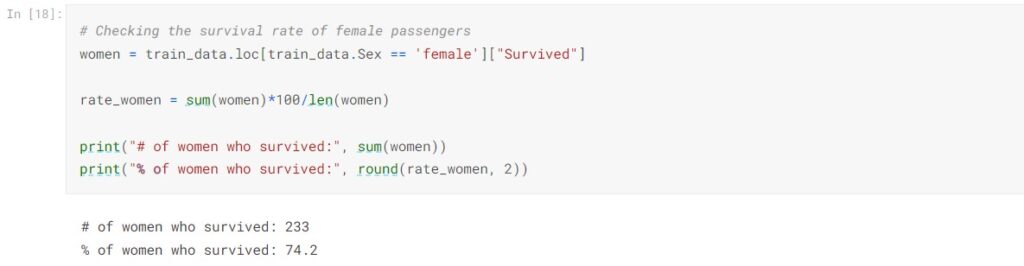
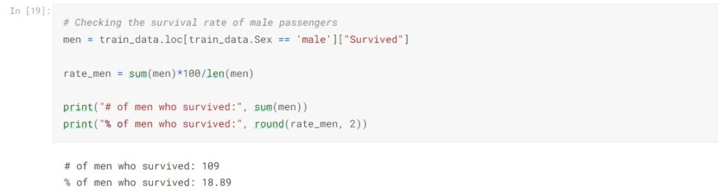
233 women and 109 men survived the shipwreck. Noticed that the female survival rate is 74.2%, which is significantly higher than males’ 18.89%. We can assume Sex will be an important feature in predicting whether the passenger would survive.
Now check the Pearson correlation coefficient of features:
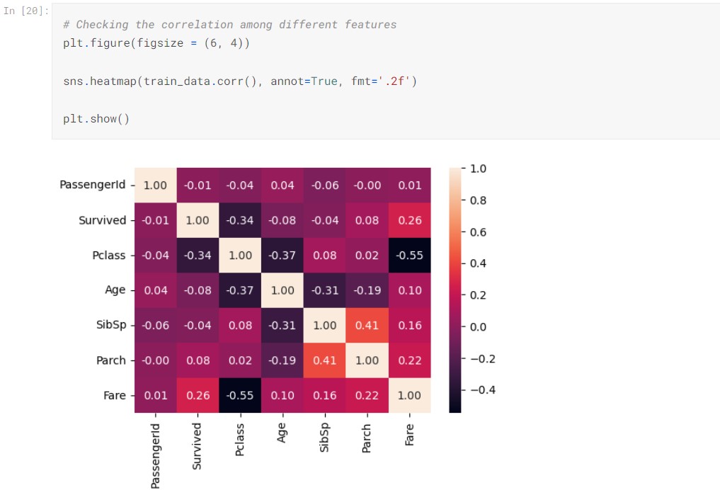
From the correlation matrix, we observed Pclass and Fare have the strongest correlation to Survived besides Sex. However, Pclass and Fare are negatively correlated having a correlation of -0.55, as higher-class ticket is cheaper. To minimize multicollinearity, we will later drop the Fare column. SibSp and Parch have some positive correlation, it suggests family tend to travel together. SibSp, Parch, and Age do not have much correlation with the survival.
EDA Summary:
- There are 891 observations and 12 columns in the train data.
- Three columns: Age, Cabin, and Embarked have missing values. Especially in Cabin 77.10% of observation is missing; In Age 19.87% of observation is missing. We will drop the Cabin column due to its high degree of absence, and we will impute the missing age with the median age. Embarked column only have 0.22% of missing value, we will impute it with the mode.
- PassengerId is the primary key in this dataset, it along with Name, Ticket will not provide much predictive power in estimating the survival of the passengers. These columns will be dropped.
- The female survival rate surpasses the male survival rate, being 74.20% and 18.89% respectively.
- Pclass and Fare are negatively correlated, 1st class and 2nd class passengers paid higher fares for their tickets. We will drop the Fare column to reduce multicollinearity.
- The survival rate decreases while the class number increases. Suggested 1st class and 2nd class passengers have higher survival rates than 3rd class passengers.
- We assume Sex and Pclass will be the most significant features in predicting the survival rate.
In the next post, I will continue the discussion and talk about data preprocessing, model building and performance evaluation.